Continuous optimization, stemming from the mathematical modeling of real-world systems, is ubiquitous in applied mathematics, operations research, and computer science. These problems often come with high dimensionality and non-convexity, posing great challenges for the design and implementation of optimization algorithms. With the advance in the fabrication of quantum computers in the past decades, extensive progress has prevailed in the pursuit of quantum speedups for continuous optimization. A conventional approach toward this end is to quantize existing classical algorithms by replacing their components with quantum subroutines, while carefully balancing the potential speedup and possible overheads. However, proposals following this approach usually achieve at most polynomial quantum speedups, and more importantly, they do not improve the quality of solutions because they essentially follow the same solution trajectories in the original classical algorithms.

Gradient descent (and its variant) is arguably the most fundamental optimization algorithm in continuous optimization, both in theory and in practice, due to its simplicity and efficiency in converging to critical points. However, many real-world problems have spurious local optima, for which gradient descent is subject to slow convergence since it only leverages first-order information. On the other hand, quantum algorithms have the potential to escape from local minima and find near-optimal solutions by leveraging the quantum tunneling effect. Therefore, it is desirable to identify a quantum counterpart of gradient descent that is simple and efficient on quantum computers while leveraging the quantum tunneling effect to escape from spurious local optima. With such features, the quality of the solutions is improved. Prior attempts (e.g., [1]) to quantize gradient descent, which followed the conventional approach, unfortunately fail to achieve the aforementioned goal, which seems to require a completely new approach to quantization.

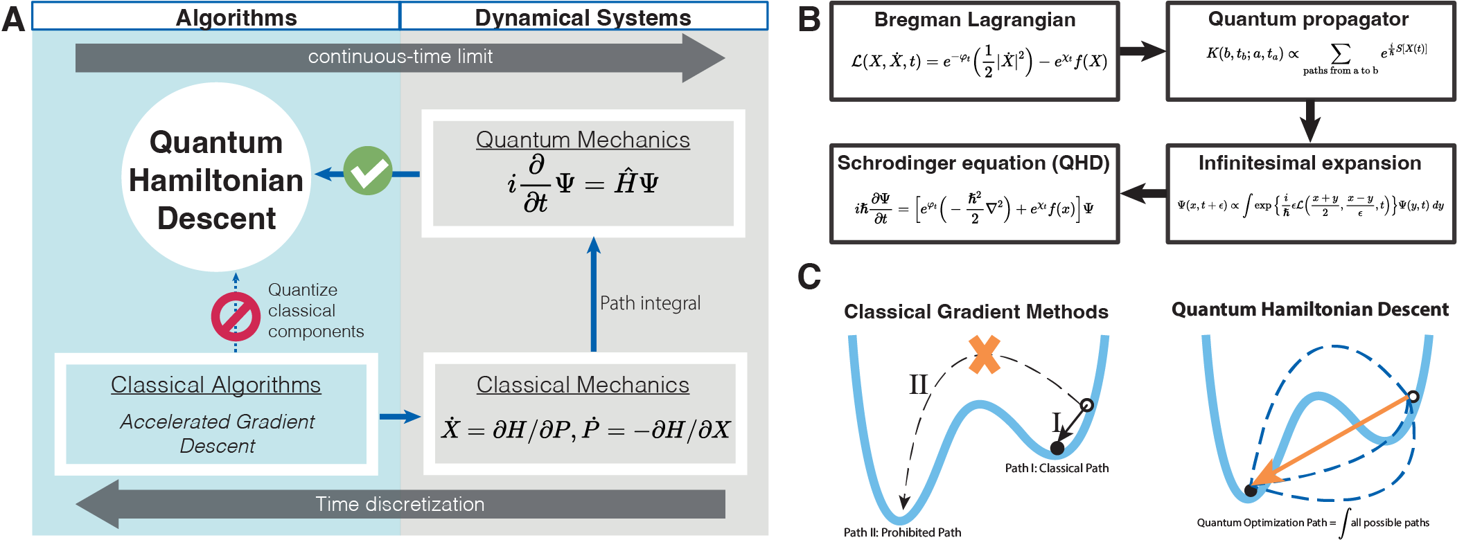
QP Comparisons — **Figure 1: Schematic of Quantum Hamiltonian Descent (QHD).** A. Road map showing the conventional and our approach of quantizing classical gradient descent (GD). Specifically, QHD is derived through the path-integral quantization of the dynamical system corresponding to the continuous-time limit of classical GD, and hence can be deemed as the path integral of the algorithmic trajectories of classical GD. B. Four major technical steps in the derivation of QHD. C. An illustrative example where classical GD with bad initialization will be trapped in a local minimum, while QHD can easily escape and find near-optimal solutions by taking the path integral of trajectories prohibited by classical mechanics.

A genuine quantum gradient descent

Our main observation is a seemingly unrelated connection between gradient descent and dynamical systems satisfying classical physical laws. Precisely, it is known that the continuous-time limit of many gradient-based algorithms can be understood as classical physical dynamical systems, e.g., the Bregman-Lagrangian framework derived in [2] to model accelerated gradient descent algorithms. Conversely, variants of gradient-based algorithms could be emerged through the time discretization of these continuous-time dynamical systems. This two-way correspondence inspired us a second approach to quantization: instead of quantizing a subroutine in gradient descent, we can quantize the continuous-time limit of gradient descent as a whole, and the resulting quantum dynamical systems lead to quantum algorithms as seen in Figure 1A. Using the path integral formulation of quantum mechanics (Figure 1B), we quantize the Bregman-Lagrangian framework to a quantum-mechanical system described by the Schrodinger equation $i \frac{d}{d t} \Psi(t) = \hat{H}(t) \Psi(t)$, where $\Psi(t)$ is the quantum wave function, and the quantum Hamiltonian reads:

\[\hat{H}(t) =e^{\varphi_t}\left(-\frac{1}{2}\Delta\right) + e^{\chi_t}f(x),~~~(1)\]

where $e^{\varphi_t}$, $e^{\chi_t}$ are damping parameters that control the energy flow in the system. We require $e^{\varphi_t/\chi_t}\to 0$ for large $t$ so the kinetic energy is gradually drained out from the system, which is crucial for the long-term convergence of the evolution. $\Delta$ is the Laplacian operator over Euclidean space, and $f(x)$ is the objective function. The Schrodinger dynamics in Eq. (1) generate a family of quantum gradient descent algorithms that we will refer to as Quantum Hamiltonian Descent, or simply QHD.

As desired, QHD inherits simplicity and efficiency from classical gradient descent. QHD takes in an easily prepared initial wave function $\Psi(0)$ and evolves the quantum system described by Eq. (1). The solution to the optimization problem is obtained by measuring the position observable $\hat{x}$ at the end of the algorithm (i.e., at time $t=T$). In other words, QHD is no different from a basic Hamiltonian simulation task, which can be done on digital quantum computers using standard techniques with provable efficiency. The simplicity and efficiency of QHD on quantum machines potentially make it as widely applicable as classical gradient descent.

For convex problems, we prove that QHD is guaranteed to find the global solution. In this case, the solution trajectory of QHD is analogous to that of a classical algorithm. Non-convex problems, known to be NP-hard in general, are much harder to solve. Under mild assumptions on a non-convex $f$, we show the global convergence of QHD given appropriate damping parameters and sufficiently long evolution time. Figure 1C shows a conceptual picture of QHD’s quantum speedup: intuitively, QHD can be regarded as a path integral of solution trajectories, some of which are prohibited in classical gradient descent. Interference among all solution trajectories gives rise to a unique quantum phenomenon called quantum tunneling, which helps QHD overcome high-energy barriers and locate the global minimum.

Performance of QHD on hard optimization problems

To visualize the difference between QHD and other classical/quantum algorithms, we test four algorithms (QHD, Quantum Adiabatic Algorithm (QAA), Nesterov’s accelerated gradient descent (NAGD), and stochastic gradient descent (SGD)) via classical simulation for 22 optimization instances with diversified landscape features selected from benchmark functions for global optimization problems.¹ QAA solves an optimization problem by simulating a quantum adiabatic evolution [3], and has been mostly applied to discrete optimization in the literature. To solve continuous optimization with QAA, a common approach is to represent each continuous variable with a finite-length bitstring so the original problem is converted to a combinatorial optimization defined on the hypercube $\{0,1\}^N$, where $N$ is the total number of bits. In our experiment, we adopt the radix-2 representation and use 7 bits for each continuous variable – this allows QAA to handle the optimization instances as discrete problems over $\{0,1\}^{14}$.²

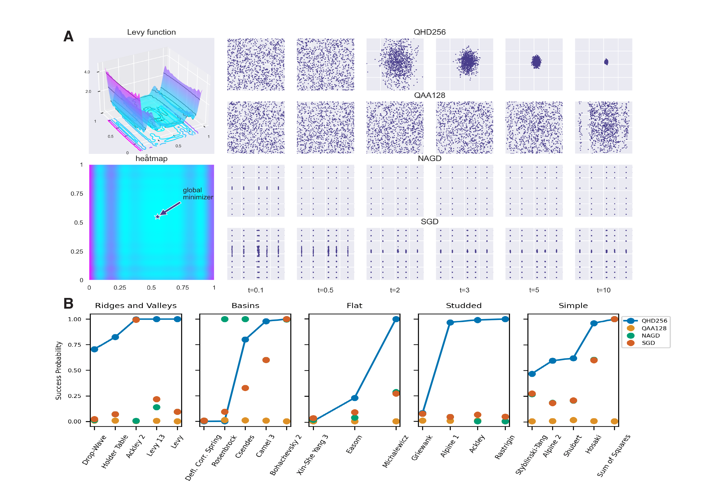
In Figure 2A, we plot the landscape of Levy function, and the solutions from the four algorithms are shown for different evolution times $t$: for QHD and QAA, $t$ is the evolution time of the quantum dynamics; for the two classical algorithms, the effective evolution time $t$ is computed by multiplying the product of learning rate and the iteration number so that it is comparable to the one used in QHD and QAA. Compared with QHD, QAA converges at a much slower rate and no apparent convergence is observed within the time window. Although the two classical algorithms seem to converge faster than quantum algorithms, they have lower success probability because many solutions have been trapped in spurious local minima. Our observation made with Levy function is consistent with the results of other functions: as shown in Figure 2B, QHD has a higher success probability in most optimization instances within the same choice of evolution time.

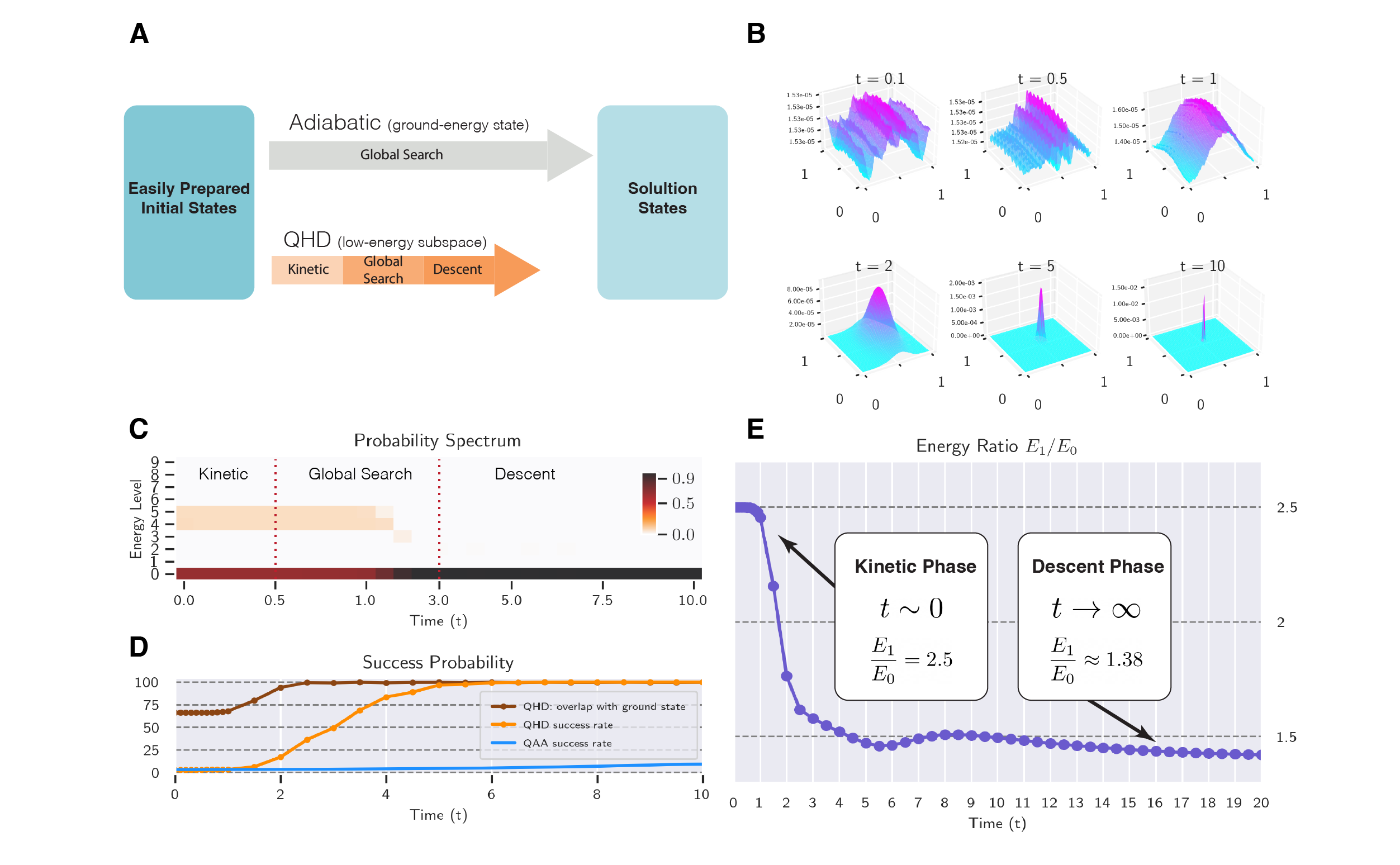
Zooming in the QHD dynamics, we find rich dynamical properties in different stages of evolution. Figure 3B shows the quantum probability densities of QHD at different evolution times: the wave function is highly oscillatory in the beginning (t = 0.1, 0.5); then, it starts moving towards the global minimum (t = 1, 2); finally, it is clustered around the global minimum and converges as like the classical gradient descent (t = 5, 10). This three-stage evolution is not only seen in Levy function, but also observed in many other instances. We thus propose to divide QHD’s evolution in solving optimization problems into three consecutive phases called the kinetic phase, the global search phase, and the descent phase according to the above observation.

The three-phase picture of QHD could be supported by a few quantitative characterizations of the QHD evolution. One such characterization is the probability spectrum of QHD, which shows the decomposition of the wave function to different energy levels (Figure 3C). QHD begins with a major ground-energy component and a minor low-energy component.³ During the global search phase, the low-energy component is absorbed into the ground-energy component, indicating that QHD finds the global minimum (Figure 3D). The energy ratio $E_1/E_0$ is another characterization of the three phases in QHD (Figure 3E), where $E_0$ (or $E_1$) is the ground (or first excited) energy of the QHD Hamiltonian $\hat{H}(t)$. In the kinetic phase, the kinetic energy $-\frac{1}{2}\Delta$ dominates in the system Hamiltonian so we have $E_1/E_0\approx 2.5$, which is the same as in a free-particle system. In the descent phase, the QHD Hamiltonian enters the ‘‘semi-classical regime’’ and the energy ratio can be theoretically computed based on the objective function.⁴

The three-phase picture of QHD sheds light on why QAA has slower convergence. Compared to QHD, QAA has neither kinetic phase nor descent phase. In the kinetic phase, QHD averages the initial wave function over the whole search space to reduce to risk of poor initialization; while QAA remains in the ground state so it never gains as much kinetic energy. In the descent phase, QHD depicts similar convergence as classical gradient descent and its convergence is insensitive to spatial resolution; such fast convergence is not seen in QAA.

From the perspective of QAA, the use of the radix-2 representation scrambles the Euclidean topology so that the resulting discrete problem is even harder than the original problem. Failed to incorporate the continuity structure, QAA is hence sensitive to the resolution of spatial discretization – we observe that higher resolutions often cause worse QAA performance.Of course, radix-2 representation is not the only way to discretize a continuous problem. One can lift QAA to the continuous domain by choosing its Hamiltonian over a continuous space in a general way. From this perspective, QHD could be possibly interpreted as a special version of the general QAA with a particular choice of the Hamiltonian. However, some existing results [4] suggest that QHD may have fast convergence that the general theory of QAA fails to explain.

Large-scale empirical study based on analog implementation

The great promise of QHD could lie in solving high-dimensional non-convex problems in real world, however, a large-scale empirical study is infeasible with classical simulation due to the curse of dimensionality. Even though theoretically efficient, an implementation of QHD instances of reasonable sizes on digital quantum computers would cost a gigantic number of fault-tolerant quantum gates,⁵, which renders any empirical study based on digital implementation a dead end for the near term.

Analog quantum computers (or quantum simulators) are alternative devices that directly emulate certain quantum Hamiltonian evolution without quantum gates, and usually have limited programmability. However, recent experimental results suggest a great advantage of continuous-time analog quantum devices over the digital ones for quantum simulation in the NISQ era due to their scalability and low overhead in simulation tasks. Compared with normal quantum algorithms that are typically described by quantum circuits, a unique feature of QHD is that its description is already a Hamiltonian simulation task by itself, which make it possible to leverage near-term analog devices for its implementation.

A conceptually simple analog implementation of QHD would be building a quantum simulator whose Hamiltonian exactly matches the QHD Hamiltonian, which is, however, not very feasible in practice. A more pragmatic strategy is to embed the QHD Hamiltonian into existing analog simulators so we can emulate QHD as part of the full dynamics. To this end, we introduce the Quantum Ising Machine (or simply QIM), as an abstract model for some of the most powerful analog quantum simulators nowadays, which is described by the following quantum Ising Hamiltonian:

\[H(t) = - \frac{A(t)}{2} \left(\sum_j \sigma^{(j)}_x\right) + \frac{B(t)}{2} \left(\sum_j h_j \sigma^{(j)}_z + \sum_{j>k} J_{j,k} \sigma^{(j)}_z \sigma^{(k)}_z\right),~~~(2)\]

where $\sigma^{(j)}_x$ and $\sigma^{(j)}_z$ are the Pauli-X and Pauli-Z operator acting on the j-th qubit, $A(t)$ and $B(t)$ are time-dependent control functions. The controllability of $A(t), B(t), h_j, J_{j,k}$ represents the programmability of QIMs, which would depend on the specific instantiation of QIM such as D-Wave systems, QuEra neutral-atom system, and so on.

At a high level, our Hamiltonian embedding technique works as follows: (i) discretize the QHD Hamiltonian Eq. (1) to a finite-dimensional matrix; (ii) identify an invariant subspace $\mathcal{S}$ of the simulator Hamiltonian for the evolution; (iii) the simulator Hamiltonian Eq. (2) is properly programmed so its restriction to the invariant subspace $\mathcal{S}$ matches the discretized QHD Hamiltonian. In this way, we effectively simulate the QHD Hamiltonian in the subspace $\mathcal{S}$ (called the encoding subspace) of the full simulator Hilbert space. By measuring the encoding subspace at the end of the analog emulation, we obtain solutions to an optimization problem.

Precisely, consider the one-dimensional case of QHD Hamiltonian that is $\hat{H}(t) = e^{\varphi_t}(-\frac{1}{2}\frac{\partial^2}{\partial x^2})+e^{\chi_t}f$. Following a standard discretization by the finite difference method, QHD Hamiltonian becomes $\hat{H}(t)= -\frac{1}{2}e^{\varphi_t}\hat{L}+e^{\chi_t}\hat{F}$ where the second-order derivative $\frac{\partial^2}{\partial x^2}$ becomes a tridiagonal matrix (denoted by $\hat{L}$), and the potential operator $f$ is reduced to a diagonal matrix (denoted by $\hat{F}$).

We identify the so-called Hamming encoding subspace $\mathcal{S}_H$ which is spanned by (n+1) Hamming states $\{\ket{H_j}:j=0,1,\dots,n\}$ for any $n$-qubit QIM. The $j$-th Hamming state $\ket{H_j}$ is the uniform superposition of bitstring states with Hamming weight (i.e., the number of ones in a bitstring) $j$:

\[\ket{H_j} = \frac{1}{\sqrt{C_j}}\sum_{|b|=j}\ket{b},\]

where $C_j$ is the number of states with Hamming weight $j$. For example, there are $n$ bitstring states with Hamming weight 1: $\ket{0\dots001}$,$\ket{0\dots010}$,…,$\ket{1\dots000}$, and the Hamming-1 state $\ket{H_1}$ is the uniform superposition of all the $n$ states. By choosing appropriate parameters $h_j$, $J_{j,k}$ in Eq. (2), the subspace $\mathcal{S}_H$ is invariant under the QIM Hamiltonian. Moreover, the restriction of the first term $\sum^r_{j=1} \sigma^{j}_x$ onto $\mathcal{S}_H$ resembles the tridiagonal matrix $\hat{L}$, and the restriction of the second term in the QIM Hamiltonian (with Pauli-Z and -ZZ operators) represents a discretized quadratic function $\hat{F}$. A measurement on $\mathcal{S}_H$ can be effectively conducted by measuring the full simulator Hilbert space in the computational basis with a simple post-processing. The Hamming encoding construction is readily generalizable to higher-dimensional Laplacian operator $\Delta$ and quadratic polynomial functions $f$.

Our Hamming encoding enables an empirical study of a self-interesting optimization problem called quadratic programming (QP) on quantum simulators. Specifically, we consider QP with box constraints:

\[\text{minimize}\qquad f(x)=\frac{1}{2} x^\top \mathbf{Q} x + \mathbf{b}^\top x,~~\text{subject to}~~\mathbf{0} \preccurlyeq x \preccurlyeq \mathbf{1},\]

where $\mathbf{0}$ and $\mathbf{1}$ are $n$-dimensional vectors of all zeros and all ones, respectively. QP problems are the simplest case of nonlinear programming and they appear in almost all major fields in computational sciences. Despite of their simplicity and ubiquity, non-convex QP problems (i.e., the Hessian matrix $\mathbf{Q}$ is indefinite) are known to be NP-hard in general.

We implement QHD on the D-Wave system⁶, which instantiates QIM and allows the control of thousands of physical qubits with decent connectivity. While existing libraries of QP benchmark instances are natural candidates for our empirical study, most of them can not be mapped to the D-Wave system because of its limited connectivity. We instead create a new test benchmark with 160 randomly generated QP instances in various dimensions (5, 50, 60, 75) whose Hessian matrices are indefinite and sparse⁷, an analog implementation of which are possible on the D-Wave machine (referred as DW-QHD).

We compare DW-QHD with 6 other state-of-the-art solvers in our empirical study: DW-QAA (baseline QAA implemented on D-Wave), IPOPT, SNOPT, MATLAB’s $\texttt{fmincon}$ (with “SQP” solver), QCQP, and a basic SciPy $\texttt{minimize}$ function (with “TNC” solver). In the two quantum methods (DW-QHD, DW-QAA), we discretize the search space $[0,1]^d$ into a regular mesh grid with 8 cells per edge due to the limited number of qubits on the D-Wave machine. To compensate the loss of the resolution, we post-process the coarse-grained D-Wave results by the SciPy $\texttt{minimize}$ function, which is a local gradient solver mimicking the descent phase of a higher-resolution QHD and only has mediocre performance by itself. The choice of classical solvers covers a variety of state-of-the-art optimization methods, including gradient-based local search (SciPy $\texttt{minimize}$, interior-point method (IPOPT), sequential quadratic programming (SNOPT, MATLAB), and heuristic convex relaxation (QCQP). Finally, to investigate the quality of the D-Wave machine in implementing QHD and QAA, we also classically simulate QHD and QAA for the 5-dimensional instances (Sim-QHD, Sim-QAA).⁸

We use the time-to-solution (TTS) metric [5] to compare the performance of solvers. TTS is the number of trials (i.e., initialization for classical solvers or shot for quantum solvers) required to obtain the correct global solution⁹ up to 0.99 success probability:

\[\text{TTS} = t_f \times \Big\lceil\frac{\ln(1-0.99)}{\ln(1-p_s)}\Big\rceil,\]

where $t_f$ is the average runtime per trial, and $p_s$ is the success probability of finding the global solution in a given trial. We run 1000 trials per instance and compute the TTS for each solver.

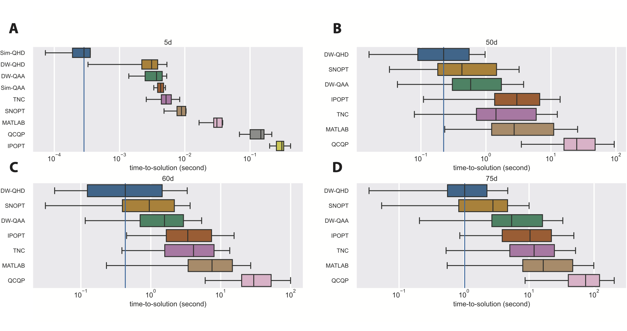
In Figure 4, we show the distribution of TTS for different solvers. We also provide spreadsheets that summarize the test results for the QP benchmark. In the 5-dimensional case (Figure 4A), Sim-QHD has the lowest TTS, and the quantum methods are generally more efficient than classical solvers. Note that, with a much shorter annealing time ($t_f=1\mu s$ for Sim-QHD and $t_f=800\mu s$ for DW-QHD), Sim-QHD still does better than DW-QHD, indicating the D-Wave system is subject to a significant load of noises and decoherence. Interestingly, Sim-QAA ($t_f=1\mu s$) is worse than DW-QAA ($t_f=800\mu s$), which shows QAA indeed has much slower convergence. In the higher dimensional cases (Figure 4B,C,D), DW-QHD has the lowest median TTS among all tested solvers. Despite of the infeasibility of running Sim-QHD in high dimensions, our observation in the 5-dimensional case suggests that an ideal implementation of QHD could perform much better than DW-QHD, and therefore all other tested solvers in high dimensions.

It is worth noting that DW-QHD does not outperform industrial-level nonlinear programming solvers such as Gurobi and CPLEX. In our experiment, Gurobi usually solves the high-dimensional QP problems with TTS no more than 0.01s. These solvers approximate the nonlinear problem by potentially exponentially many linear programming subroutines and use a branch-and-bound strategy for a smart but exhaustive search of the solution.¹⁰ However, the restriction of the D-Wave machine (e.g., programmability and decoherence) forces us to test on very sparse QP instances, which can be efficiently solved by highly-optimized industrial-level branch-and-bound solvers. On the other side, we believe that QHD should be more appropriately deemed as a quantum upgrade of classical GD, which would more conceivably replace the role of GD rather than the entire branch-and-bound framework in classical optimizers.

Conclusions

In this work, we propose Quantum Hamiltonian Descent as a genuine quantum counterpart of classical gradient descent through a path-integral quantization of classical algorithms. Similar to classical GD, QHD is simple and efficient to implement on quantum computers; meanwhile, it leverages the quantum tunneling effect to escape from spurious local minima, which we believe could replace the role of classical GD in many optimization algorithms. Moreover, with the newly developed Hamiltonian embedding technique, we conduct a large-scale empirical study of QHD on non-convex quadratic programming instances up to 75 dimensions, via an analog implementation of QHD on the D-Wave instantiation of a quantum Ising Hamiltonian simulator. We believe that QHD could be readily used as a benchmark algorithm for other quantum or semi-quantum analog devices, for testing the quality of the devices and conducting more empirical study of QHD.

References

[1] Patrick Rebentrost, Maria Schuld, Leonard Wossnig, Francesco Petruccione, and Seth Lloyd, Quantum gradient descent and newton’s method for constrained polynomial optimization, New Journal of Physics 21 (2019), no. 7, 073023.

[2] Andre Wibisono, Ashia C Wilson, and Michael I Jordan, A variational perspective on accelerated methods in optimization, Proceedings of the National Academy of Sciences 113 (2016), no. 47, E7351–E7358.

[3] Edward Farhi, Jeffrey Goldstone, Sam Gutmann, Joshua Lapan, Andrew Lundgren, and Daniel Preda, A quantum adiabatic evolution algorithm applied to random instances of an NP-complete problem, Science 292 (2001), no. 5516, 472–475.

[4] Gheorghe Nenciu, Linear adiabatic theory: exponential estimates, Communications in Mathematical Physics 152 (1993), no. 3, 479–496.

[5] Troels F Rønnow, Zhihui Wang, Joshua Job, Sergio Boixo, Sergei V Isakov, David Wecker, John M Martinis, Daniel A Lidar, and Matthias Troyer, Defining and detecting quantum speedup, Science 345 (2014), no. 6195, 420–424.

Footnotes