In this benchmark test, we compare QHD run on the D-Wave Advantage 6.1 system with the standard quantum adiabatic algorithm, UCSD’s SNOPT, COIN-OR’s IPOPT, MATLAB’s fmincon, QCQP, and SciPy’s minimize on four sets of randomly generated quadratic programming problems of various dimensions (5d, 50d, 60d, 75d). QHD compares favorably with both classical local solvers and the native quantum annealing algorithm of the D-Wave device.
Problem Formulation
In our experiment, we consider quadratic programming problems with box constraints:
\(\text{minimize}~~\frac{1}{2} x^T Q x + b^T x \ \ \text{s.t.},\ \ 0 \leq x \leq 1\).
Methodology
We randomly generate instances of dimension 5, 50, 60, 75 and compare the performance of multiple methods and solvers. Due to the limited connectivity and number of qubits, the maximum dimension of the problems we are able to embed on the D-Wave QPU is roughly 75. To create the problems we uniformly sample entries for the Hessian matrices \(Q\) on \([0,1]\) with pentadiagonal structure in order to fix a maximum sparsity. This makes a minor embedding possible so that the problem can be run on the D-Wave QPU.
For each of problem sets, we compare the performance of six methods (see “Comparisons” in Details): QHD on D-Wave, QAA on D-Wave, IPOPT, SNOPT, MATLAB’s fmincon with SQP, QCQP, and a SciPy’s minimize.
For the classical methods, the initial points are drawn uniformly at random from \([0,1]^d\).
We use the time-to-solution (TTS) metric to compare the performance of solvers. TTS is the number of trials (i.e., initialization for classical solvers or shot for quantum solvers) required to obtain the correct global solution up to 0.99 success probability:
\[\text{TTS} = t_f \times \Big\lceil\frac{\ln(1-0.99)}{\ln(1-p_s)}\Big\rceil,\]
where \(t_f\) is the average runtime per trial, and \(p_s\) is the success probability of finding the global solution in a given trial. We run 1000 trials per instance and compute the TTS for each solver. Clearly, lower TTS means better performance for an optimization solver.
Results
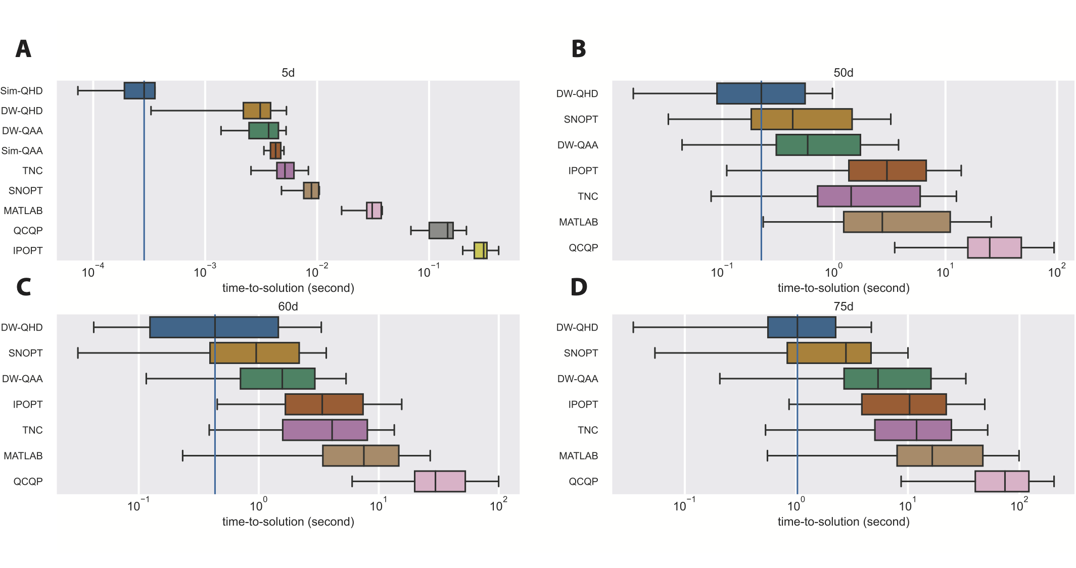
In the above figure, we show the distribution of TTS for different solvers. We also provide spreadsheets that summarize the test results for the QP benchmark. In the 5-dimensional case (Panel A), Sim-QHD has the lowest TTS, and the quantum methods are generally more efficient than classical solvers. Note that, with a much shorter annealing time (\(t_f=1\mu s\) for Sim-QHD and \(t_f=800\mu s\) for DW-QHD), Sim-QHD still does better than DW-QHD, indicating the D-Wave system is subject to a significant load of noises and decoherence. Interestingly, Sim-QAA (\(t_f=1\mu s\)) is worse than DW-QAA (\(t_f=800\mu s\)), which shows QAA indeed has much slower convergence. In the higher dimensional cases (Panel B,C,D), DW-QHD has the lowest median TTS among all tested solvers. Despite of the infeasibility of running Sim-QHD in high dimensions, our observation in the 5-dimensional case suggests that an ideal implementation of QHD could perform much better than DW-QHD, and therefore all other tested solvers in high dimensions.
For more discussions, see “Large-scale empirical study based on analog implementation” in Executive Summary.